Introduction

Wouldn't it be great if the cryptocurrency markets just kept going up and up and up? Sounds sweet right? But that is never the case since "nothing lasts forever" and no market rises forever. "What goes up must come down," and this is true for all financial markets as well.

We have seen enormous gains when the crypto markets move upwards, but we have also witnessed significant losses when they move in the opposite way, i.e. downwards. When the market crashes, asset prices fall, giving investors the opportunity to purchase these assets at a discount. We may also add that as prices dip, investors buy, thus the phrase "Buy the Dip."

What is "Buy the Dip"?

Buy the Dip is an investing strategy where an investor buys a particular asset whenever the price of an asset falls. When an investor Buys the Dip, it signifies that the investor has faith in the asset, these price corrections are temporary, and the asset has the potential to generate significant returns over a period of time.

In our case, we will buy Bitcoin (BTC) worth $10 whenever the BTC falls below 5%.

Strategy

We will begin implementing this strategy from after the covid crash, which occurred on March 16, 2020.

• Whenever the price of the asset (BTC) goes below 5% we will buy, else won't buy.
• We will sell our BTC holdings 3 weeks after the BTC November top (likely)
• We will sell our BTC holdings at the November top (unlikely)
• We will keep on accumulating BTC and hodl (unrealised)

Libraries Used

The libraries used in this project make it extremely simple to analyze your data. Installing these libraries is done using the pip command in the terminal:

pip install library_name

The libraries used are briefly described below:

• Pandas - To easily manipulate data in a dataframe
• Numpy - To visualize your data
• Matplotlib - To make numerical calculations within a grouped data simple
• Requests - Used for making HTTP requests
• Datetime - To perform operations on dates

Lets Begin Coding!!

Importing Libraries

import pandas as pd
import requests
import matplotlib.pyplot as plt
from datetime import datetime
import numpy as np

Extracting Data

To extract the data, in this project we will use the Glassnode API.

API Key and URL

To access the Glassnode API, you will require an API key. You can get an API key and use glassnodes basic services for free by signing up for a Glassnode account by clicking here.

To know more about how to get the API key, click here.

api_key="API_KEY" #your API Key
url='https://api.glassnode.com/v1/metrics/market/price_usd_close' #metrics we require

To know more about the url link used in the above code click here.

Glassnode, "provides the data, knowledge, and confidence to make better investment and trading decision in Bitcoin, Ethereum and cryptocurrency markets." You may use the Glassnode API to retrieve a number of metrics such as on-chain data, derivatives data and much more which you could use in your other projects.

Get Request

Once we have our required URL, we can continue to get our required data.

res=requests.get(url,params={'a':'BTC', 's':1584297000,'api_key':api_key})
data=pd.read_json(res.text,convert_dates=['t']) #converting data from json to dataframe

Parameters used: a-asset, s-date in epoch format and api_key - API key. To know about the other parameters, click here. The parameter, convert_dates=['t'] converts date column from epoch to datetime format.

You can use this site to convert date to epoch format or vice versa. 1584297000 in date format is 15th March, 2020.

Please feel free to explore the Glassnode API by clicking here. The Glassnode API is a very simple and easy to use API that explains all of the API features in a straightforward manner.

Viewing our Data

data.head()

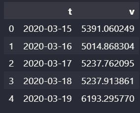
The .head() function returns the top 5 rows of our dataframe. We can get a brief overview of our data using this function.

In the output for the above code, we can notice our date and price column are labelled 't' and 'v' respectively. We will change it to "Date" and "Price USD" in the "Working on Data" section.

Cleaning Data

Data when extracted, can be having null values, duplicate value and the data maybe even of the wrong datatype. We need to check this since, bad data will give us inaccurate results.

Checking Datatypes

data.dtypes

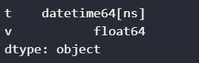
This function returns the datatype of our dataframe columns. We can notice, the 't' column and our 'v' column have the correct datatype of datetime and float.

Checking Null and Duplicate Values

print(data.isna().sum().sum())
print(data.duplicated().sum())

For the above code, we get our output as 0 and 0 indicating there are no Null or duplicate values present.

Working on Data

Changing Column Names

As we have seen above, are column names are 't' and 'v'. This will be changed so that we can have a better understanding of our data.

data.columns=['Date','Price USD']

If we run the .head function, you will notice the columns of your dataframe is changed.

Adding Percentage Change column

How will we know if BTC dipped below 5%? - By finding the daily percentage change of BTC, by using the pct_change function.

data['Percentage Change']=data['Price USD'].pct_change()

After executing the above code, if we run the .head function, you will notice a new column, "Percentage Change" in your dataframe which will have the daily percentage change of BTC.

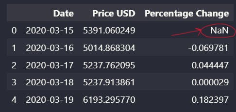
We can also see the first row in the "Percentage Change" column is a Null value. Hence, we need to drop this.

data.dropna(inplace=True)

Since we dropped this value, our first row now will have the index 1 (try running .head function). Rows index always start from 0 hence, we need to reset our index.

data.reset_index(drop=True, inplace=True)

After running the above code, our row index begins from 0. We can plot our data and begin our analysis.

Plotting Our Data

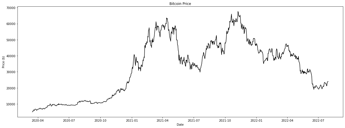
Plotting Bitcoin's Price overtime

plt.figure(figsize=(20,7))
plt.plot(data['Date'],data['Price USD'],color='black')

plt.title("Bitcoin Price")
plt.xlabel("Date")
plt.ylabel("Price ($)")

plt.plot()
plt.show()

Plotting Bitcoin's Price with Daily Percent Change

x=data['Date']
y1=data['Price USD']
y2=data['Percentage Change']

plt.rcParams["figure.figsize"] = (20,7)
fig, ax1=plt.subplots()
ax2=ax1.twinx()

ax1.plot(x,y1,label="Price",color='black')
ax2.plot(x,y2,label="Percentage Change",color='orange')

ax1.set_xlabel("Date")
ax1.set_ylabel("Price USD")
ax2.set_ylabel("Percentage Change")

h1, l1 = ax1.get_legend_handles_labels()
h2, l2 = ax2.get_legend_handles_labels()
ax1.legend(handles=h1+h2, labels=l1+l2, loc='upper left')

plt.title("Price Vs Percentage Change")
plt.plot()
plt.show()

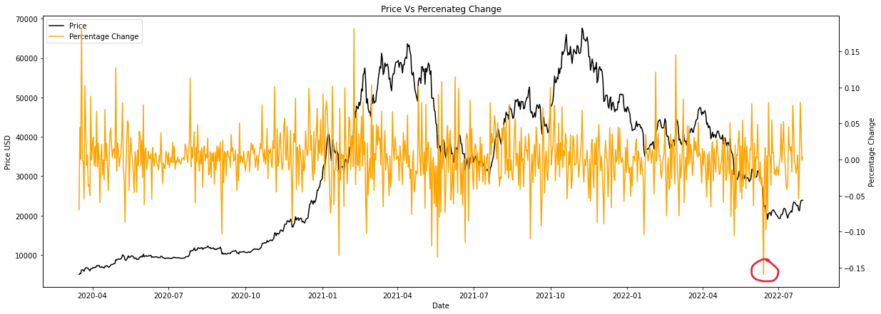
From our output, we can notice one of the biggest daily percentage change (-15%) of BTC took place recently, which was around in June, 2022.

Selling Three Weeks after the Top

BTC topped out on November 8th, 2021 hence 3 weeks after that will be 29th November 2021. Hence, we need to find the price of BTC on 29-11-2021 as we are selling our holdings that day.

Finding BTC Price 3 weeks after top

sell_price1=0  #stores our selling price
for i in range (len(data)):
    a=data.loc[i,'Date']  #stores date
    if datetime.strftime(a, "%Y-%m-%d")=='2021-11-29':  #converting "datetime" datatype to "string"
        sell_price1=data.loc[i,'Price USD']
        break

Finding the number of times the Percentage Change of BTC was below 5%

q1=0 #Quantity of BTC 
c1=0 #number of times the percentage change of BTC was below 5% 

for i in range(len(data)):

    pct=data.loc[i,'Percentage Change']
    a=data.loc[i,'Date']

    if datetime.strftime(a, "%Y-%m-%d")=='2021-11-29':
        break

    if pct <= -0.05:
        c1+=1
        price=data.loc[i,'Price USD']
        q1=q1+(10/price)

Calculations

amt_invested1=10*c1

avg_price1=amt_invested1/q1

value_sold1=sell_price1*q1
profit_loss1= value_sold1-amt_invested1

roi1=(profit_loss1/amt_invested1)*100

Displaying Results

print("Number of recurring buys -",c1)

print("\nQuantity of BTC bought",q1,'BTC')

print("\nAverage Buying Price -> $",avg_price1)
print("Selling Pirce -> $",sell_price1)

print("\nAmount Invested -> $",amt_invested1)
print("Portfolio Value when sold -> $",value_sold1)

print("\nProfit/Loss -> $",profit_loss1)
print("ROI ->",roi1,'%')

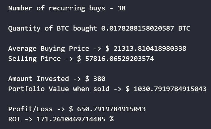
From our above results, we notice the daily percentage change of BTC fell below 5% 38 times between the periods of March 16, 2020 and 29th November 2021. If we bought BTC during these times, we could have made an ROI of over 150% which is 1.5x your investment.

Selling at the Top

This is one of the most unlikeliest scenarios since no one can predict the top or bottom of any market.

Finding Top Selling Price and Top Price Date

top_sell_price=max(data['Price USD'])

top_date=''

for i in range(len(data)):
    if data.loc[i,'Price USD']==top_sell_price:
        top_date=data.loc[i,'Date']
        break

Finding the number of times the Percentage Change of BTC was below 5%

q2=0 #Quantity of BTC 
c2=0 #number of times the percentage change of BTC was below 5% 

for i in range(len(data)):

    pct=data.loc[i,'Percentage Change']
    a=data.loc[i,'Date']

    if a==top_date:
        break

    if pct <= -0.05:
        c2+=1
        price=data.loc[i,'Price USD']
        q2=q2+(10/price)

Calculations

amt_invested2=10*c2

avg_price2=amt_invested2/q2

sell_price2=top_sell_price*q2

profit_loss2= sell_price2-amt_invested2

roi2=(profit_loss2/amt_invested2)*100

Displaying Results

print("Number of recurring buys -",c2)

print("\nQuantity of BTC bought",q2,'BTC')

print("\nAverage Buying Price -> $",avg_price2)
print("Selling Pirce -> $",top_sell_price)

print("\nAmount Invested -> $",amt_invested2)
print("Portfolio Value when sold -> $",sell_price2)

print("\nProfit/Loss -> $",profit_loss2)
print("ROI ->",roi2,'%')

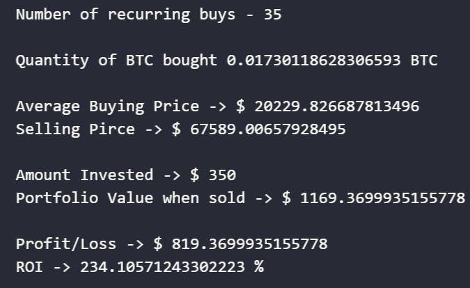
From our above results, we notice the daily percentage change of BTC fell below 5% 35 times between the periods of March 16, 2020 and 8th November 2021. If we bought BTC during these times, we could have made an ROI of over 200% which is 2x your investment.

HODL

In this scenario, we will continue to buy BTC and not sell our holdings.

Finding the number of times the Percentage Change of BTC was below 5%

q3=0 #Quantity of BTC 
c3=0 #number of times the percentage change of BTC was below 5% 

buying_prices=[]

for i in range(len(data)):
    pct=data.loc[i,'Percentage Change']

    if pct <= -0.05:
        c3+=1
        price=data.loc[i,'Price USD']
        q3=q3+(10/price)

Calculations

amt_invested3=10*c3

avg_price3=amt_invested3/q3

current_BTC_value=data.loc[852,'Price USD'] #today's BTC price

unrealised=current_BTC_value*q3

profit_loss3= unrealised-amt_invested3

roi3=(profit_loss3/amt_invested3)*100

Displaying Results

print("Number of recurring buys -",c3)

print("\nQuantity of BTC bought",q3,'BTC')

print("\nAverage Buying Price -> $",avg_price3)
print("Current Pirce -> $",current_BTC_value)

print("\nAmount Invested -> $",amt_invested3)
print("Current Balance -> $",unrealised)

print("\nUnlrealised Profit/Loss -> $",profit_loss3)
print("ROI ->",roi3,'%')

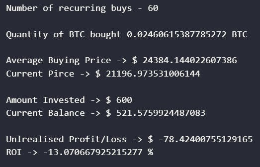
From our above results, we notice the daily percentage change of BTC fell below 5% 35 times between the periods of March 16, 2020 and now. If we bought BTC during these times, we could have made an unrealised ROI of over -13%.

Analyzing all 3 Scenarios (Data Visualization)

Int this section, we will compare the results of our three scenarios visually.

Storing our results in a list

We will store our results into lists in order to visualize our results in a simple manner.

strategy=['Scenario1','Scenario2','Scenario3']
avg_buying_price=[avg_price1,avg_price2,avg_price3]
amt_invested=[amt_invested1,amt_invested2,amt_invested3]

qty=[q1,q2,q3]

profit_loss=[profit_loss1, profit_loss2, profit_loss3]
roi=[roi1,roi2,roi3]

Comparing Amount Invested and Profit/Loss

x_axis = np.arange(len(strategy))

plt.figure(figsize=(10,7))
plt.bar(x_axis -0.2, amt_invested, width=0.4, label = 'Amount Invested')
plt.bar(x_axis +0.2, profit_loss, width=0.4, label = 'Profit/Loss')

plt.xticks(x_axis, strategy)

plt.legend()

plt.title("Amount Invested Vs Profit/loss")
plt.show()

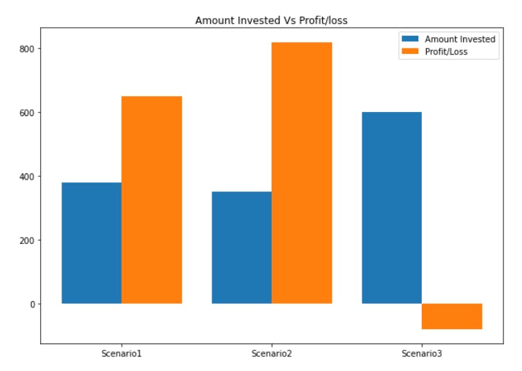From the above output, we can notice Scenario 2 - which is the most unlikeliest to happen scenario since no one can predict the top or bottom, gives the greatest Profit, followed by Scenario1 and then Scenario 3 which is in loss.

Scenario 3 has the most amount invested since we are still accumulating (buying) more BTC.

Comparing ROI

plt.figure(figsize=(10,7))
plt.bar(strategy,roi)

plt.ylabel("ROI")
plt.title("ROI")

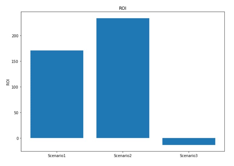We can notice, the ROI for Scenario 3 is the highest, followed by Scenario 1 and Scenario 3.

Comparing Quantity of BTC Accumulated

plt.figure(figsize=(10,7))
plt.bar(strategy,qty,color='gold')

plt.ylabel("BTC")
plt.title("Quantity of BTC Accumulated")

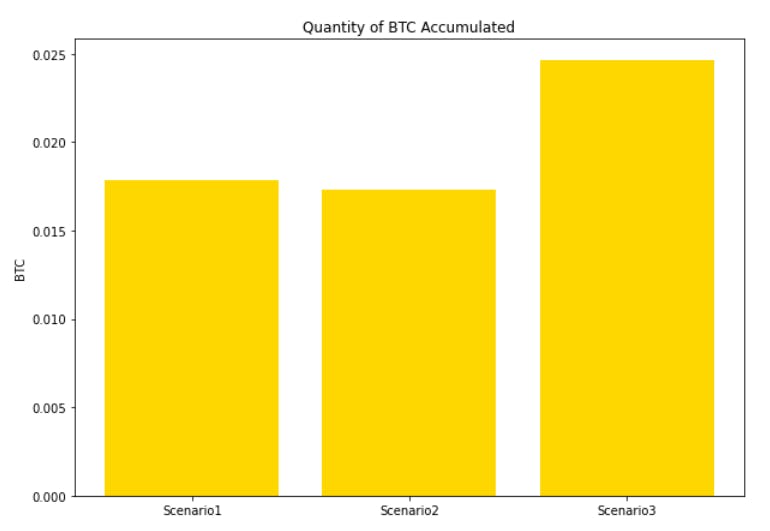
Scenario 3 has the highest quantity of BTC accumulated since, our investing period in the Scenario 3 is longer as compared to Scenario 1 and 2.

Comparing Average Buying Price

plt.figure(figsize=(10,7))
plt.bar(strategy,avg_buying_price,color='pink')

plt.ylabel("$")
plt.title("Average Buying Price")

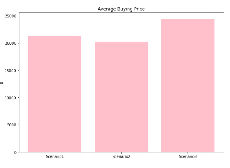Despite Scenario 3 currently being in loss, we can notice the average buying price of our investment is just slightly higher that Scenario 1 and 2.

Conclusion

"Buy the Dip" is just one of the many investing strategies out there, which may have the potential to make an investor significant gains (which we have seen above). However, this is NOT financial advise; all work done here is entirely for educational purposes. Before investing, an investor should perform their own research. An investor, can combine this strategy with other strategies to achieve even greater results.

Furthermore, feel free to try this code with a number of cryptocurrencies such as Ethereum, Solana, Binance and many more. You may also increase the amount invested each time to $50, $100.. and may also increase the daily percentage change to maybe 8%, 10%, 15% and so on. Meaning, you may buy $50 worth of a particular cryptocurrency when the daily percentage change falls below 10%.

Please mention your results in the comments below.

Key Takeaways

• We have gathered data using Glassnode API.
• Next, we checked if the data is free from errors.
• We then, began our analysis.
• We obtain the results for our three scenarios and then visualize them.
• From our analysis, Scenario 2 has the greatest ROI, followed by Scenario 1, and then Scenario 3 (unrealised ROI).
• Scenario 2 is the most unlikeliest to happen since no one can predict the top or bottom of a market.
• This is NOT FINANCIAL ADVICE.

Please feel free to connect with me and ask for any investing strategy or analysis you'd like me to perform. If you enjoyed my article and found it informative please follow and comment below. Thank you for your time.