


Introduction
Global financial markets are in the red due to a variety of macroeconomic factors. Despite the fact that many investors have lost a lot of money during this period, many investors feel that the current bear market has the potential to create generational wealth since the prices of a number of blue chip assets are so low.
What is DCA?
DCA stands for "Dollar Cost Averaging", it is a type of investing strategy where you invest a fixed amount of capital to buy an asset regardless the price of the asset on a specific date such as weekly, monthly.
In this blog, we go through three scenarios (strategies), after which we will then compare the returns of DCAing $10 in Bitcoin every Sunday.
Scenario 1:
Accumulate Bitcoin only through bear market and sell after bull market tops out.
Scenario 2:
Accumulate Bitcoin throughout the Bull Market and sell after the bull market tops out.
Scenario 3:
Continue accumulating Bitcoin during the Bear and Bull markets and sell after the bull market tops out.
Since no one can predict the top or bottom of the market, we will start accumulating 3 weeks after the top and 3-4 weeks after the bottom.
When to Buy/Sell?
Before beginning, we have to figure out when do we start buying and when do we start selling Bitcoin. To do so, we will check out the trading view chart of Bitcoin and find the dates of when to buy and sell. I have used this chart.
If you do not have a trading view account, you can signup by clicking here. - By doing so, if you decide to upgrade to a premium plan, you will receive a reward of up to $30.
Buying Dates
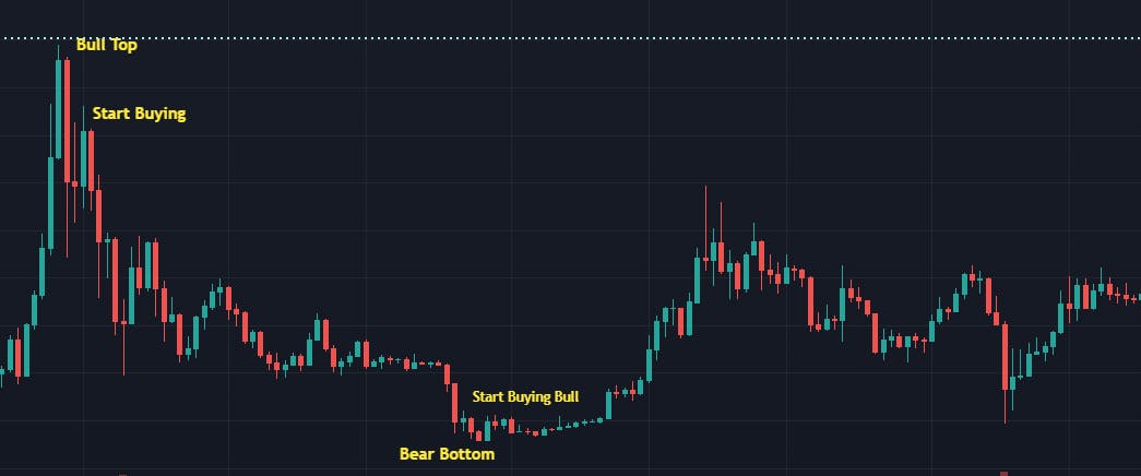
In the above chart, we can notice the Bull Market of 2017 topped out on 11th December 2017, the top price was $19802. Hence, 4 weeks after the top we will get our date as the 7th of January, 2018. This is when we will begin buying BTC as specified in Scenario 1 and Scenario 3.
We also can notice the Bear Market Bottom in the above chart which bottomed out on the 10th of December 2018, the bottom price was $3218. Hence, 4 weeks from this bottom we get our date as 1st January, 2019. This is when we will begin buying BTC as specified in Scenario 2.
Selling Dates
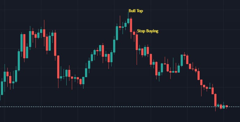
In the above chart, we can notice the Bull Market of 2021 topped out on 8th November 2021, the top price was $68000. Hence, 3 weeks after the top we will get our selling date as 29th November 2021. This is when, we will sell all out BTC holdings as specified in Scenario 1, Scenario 2 as well as Scenario 3.
Libraries Used
The libraries used in this project make it extremely simple to analyze your data. Installing these libraries is done using the pip command in the terminal:
pip install library_name
The libraries used are briefly described below:
- Pandas - To easily manipulate data in a dataframe
- Matplotlib - To visualize your data
- Numpy - To make numerical calculations within grouped data simple
- Coinmetrics.api_client - To get the required data (Bitcoin Price data)
- datetime - To perform operations on dates
- calendar - To find which date is Sunday
Lets Begin Coding!!
Importing the required libraries
import pandas as pd
from coinmetrics.api_client import CoinMetricsClient
import datetime as dt
import matplotlib.pyplot as plt
import calendar
from datetime import datetime
import numpy as np
Importing Data
client = CoinMetricsClient()

asset='btc' #bitcoin
start_time='2018-01-07' #the date 4 weeks after bull market tops
end_time=dt.datetime.today() #returns todays date

metrics_list = ['PriceUSD'] #metrics we require

df = client.get_asset_metrics(
  assets=asset, metrics=metrics_list, start_time=start_time, end_time=end_time).to_dataframe() #converting the data into a dataframe
Coinmetrics "organizes the world’s crypto data and makes it transparent and accessible." The CoinMetrics API provides you with a number of metrics such as on-chain metrics, exchange metrics, asset metrics and much more which you can include in your projects.
To know more about the CoinMetricsClient API, click here and here. Feel free to checkout the CoinMetrics API docs, which makes using an API very simple and is very easy to understand.
Viewing Data
df.head()
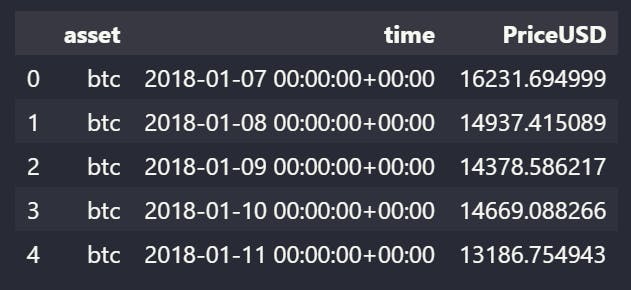 This function, returns the first 5 rows of your dataframe. By executing the .head() function, you can get a brief overview over the data you are working on.
Checking for Bad Data (Data Cleaning)
Null and Duplicate Values
print(df.isna().sum().sum())   #returns sum of null values in dataframe
print(df.duplicated().sum().sum())   #returns sum of duplicate values in dataframe
The output of the above code will be 0, indicating there are neither Null nor Duplicate values present in our dataframe.
Datatypes of the Metrics
df.dtypes
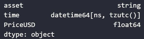 The datatype of each column in the dataframe will be returned by the code above. We can see that the datatype of each metric is correct, hence no datatype changes are required.
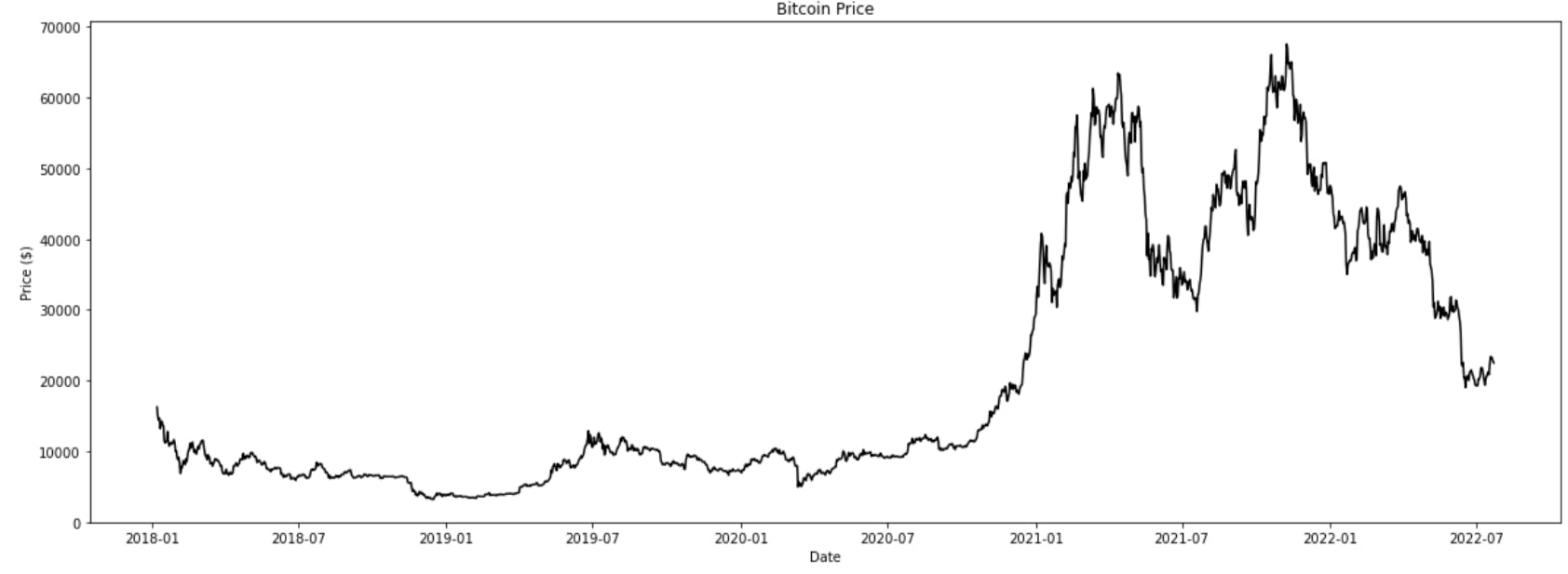
Plotting Bitcoin's Price overtime
plt.figure(figsize=(20,7))
plt.plot(df['time'],df['PriceUSD'],color='black')

plt.title("Bitcoin Price")
plt.xlabel("Date")
plt.ylabel("Price ($)")

plt.plot()
plt.show()
Finding Selling Price
As we know, we are selling out Bitcoin holdings 3 weeks after the top which is '2021-11-29'. We need to find the price on this date.
top_sell_price=0
for i in range (len(df)):
    a=df.loc[i,'time']
    if datetime.strftime(a, "%Y-%m-%d")=='2021-11-29':
        top_sell_price=df.loc[i,'PriceUSD']
        break
top_sell_price will store our selling price, .loc[i,'time'] function stores the date of each row in the dataframe, datetime.strftime function converts datatype from 'datatime' to 'string'.
After executing the above code, we get our top_selling_price value as $57920.7107299825.
Scenario 1
In Scenario 1, we begin accumulating BTC from '2018-01-07' up to '2019-01-07' that is during the bear market.
qty1=0  #stores quantity of BTC accumulated
c1=0  #stores count of number of Sundays

for i in range(len(df)):
    a=df.loc[i,'time']
    if calendar.day_name[a.weekday()]=='Sunday':
        price=df.loc[i,'PriceUSD']
        c1+=1
        qty1=qty1+(10/price)

    if datetime.strftime(a, "%Y-%m-%d")=='2019-01-07':
        break
The function, calendar.day_name[a.weekday()] converts the given date to its weekday. In the quantity statement, qty1=qty1+(10/price) we use 10 since we are investing $10 in BTC every Sunday.
Scenario 1 Calculations
amt_invested1=c1*10  #total amount invested number of sundays * 10

avg_buying_price1=amt_invested1/qty1 #average BTC buying price

sell_price1=top_sell_price*qty1  #Investment value after selling

profit_loss1=sell_price1-amt_invested1

roi1=(profit_loss1/amt_invested1)*100  #Return on Investment
Scenario 1 Results
print("Quantity Accumulated during Bear Market -",qty1,"BTC")

print("\nAmount Invested - $",amt_invested1)
print("Average BTC Buying Price - $",avg_buying_price1)

print("\nSelling Value - $",sell_price1)

print("\nRealised Profit/Loss - $",profit_loss1)
print("ROI -",roi1,"%")
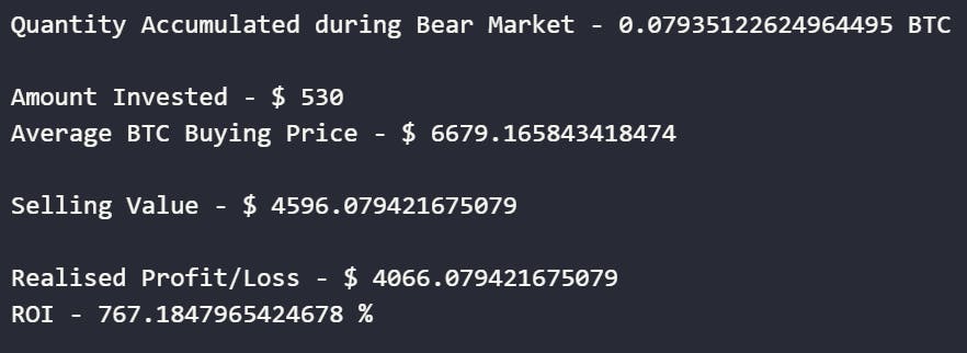
We can notice, by just accumulating BTC in the bear market we have made an ROI of over 750% which is 7.5x your investment.
Furthermore, to get precise value, we can use the round() function and round up the value up to how many ever decimal places you prefer.
Scenario 2
In Scenario 2, we begin accumulating BTC from '2019-01-07' up to '2021-11-29' that is during the Bull Market.
qty2=0 #stores quantity of BTC accumulated
c2=0  #stores count of number of Sundays

for i in range(index,len(df)):
    a=df.loc[i,'time']
    if calendar.day_name[a.weekday()]=='Sunday':
        price=df.loc[i,'PriceUSD']
        qty2=qty2+(10/price)
        c2+=1

    if datetime.strftime(a, "%Y-%m-%d")=='2021-11-29':
        break
Scenario 2 Calculations
amt_invested2=c2*10

avg_buying_price2=amt_invested2/qty2

sell_price2=top_sell_price*qty2

profit_loss2=sell_price2-amt_invested2

roi2=(profit_loss2/amt_invested2)*100
Scenario 2 Results
print("Quantity Accumulated during Bull Market ->",qty2,"BTC")

print("\nAmount Invested -> $",amt_invested2)
print("Average BTC Buying Price -> $",avg_buying_price2)

print("\nSelling Value -> $",sell_price2)

print("\nRealised Profit/Loss -> $",profit_loss2)
print("ROI ->",roi2,"%")
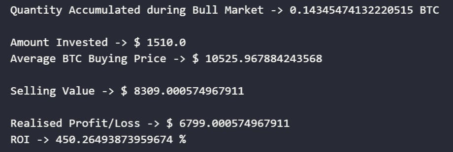
We can notice, by just accumulating BTC in the bull market we have made an ROI of 450% which is 4.5x your investment.
Scenario 3
In Scenario 3, we begin accumulating BTC from '2018-01-07' until we sell at top '2021-11-29' which is during the bear and bull market.
qty3=0#stores quantity of BTC accumulated
c3=0  #stores count of number of Sundays

for i in range(len(df)):
    a=df.loc[i,'time']
    if calendar.day_name[a.weekday()]=='Sunday':
        price=df.loc[i,'PriceUSD']
        qty3=qty3+(10/price)
        c3+=1

    if datetime.strftime(a, "%Y-%m-%d")=='2021-11-29':
        break
Scenario 3 Calculations
amt_invested3=10*c3

avg_buying_price3=amt_invested3/qty3

sell_price3=top_sell_price*qty3

profit_loss3=sell_price3-amt_invested3

roi3=(profit_loss3/amt_invested3)*100
Scenario 3 Results
print("Quantity Accumulated during Bear and Bull Market ->",qty3,"BTC")

print("\nAmount Invested -> $",amt_invested3)
print("Average BTC Buying Price -> $",avg_buying_price3)

print("\nSelling Value -> $",sell_price3)

print("\nRealised Profit/Loss -> $",profit_loss3)
print("ROI ->",roi3,"%")
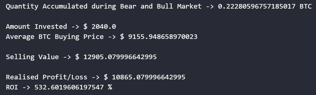
We can notice, by accumulating BTC during the bull and bear market, we have made an ROI of over 500% which is 5x your investment.
Comparing all three Scenarios (Data Visualization)
Storing our results in a list to visualize
strategy=['Scenario1','Scenario2','Scenario3']
avg_buying_price=[avg_buying_price1,avg_buying_price2,avg_buying_price3]
amt_invested=[amt_invested1,amt_invested2,amt_invested3]
qty=[qty1,qty2,qty3]
profit_loss=[profit_loss1, profit_loss2, profit_loss3]
roi=[roi1,roi2,roi3]
Visualizing Amount Invested and Profit/Loss
plt.figure(figsize=(7,5))

x_axis = np.arange(len(strategy))

plt.bar(x_axis -0.2, amt_invested, width=0.4, label = 'Amount Invested')
plt.bar(x_axis +0.2, profit_loss, width=0.4, label = 'Profit/Loss')

plt.xticks(x_axis, strategy)

plt.legend()
plt.title("Amount Invested and Profit/Loss")
plt.ylabel("$")
plt.show()
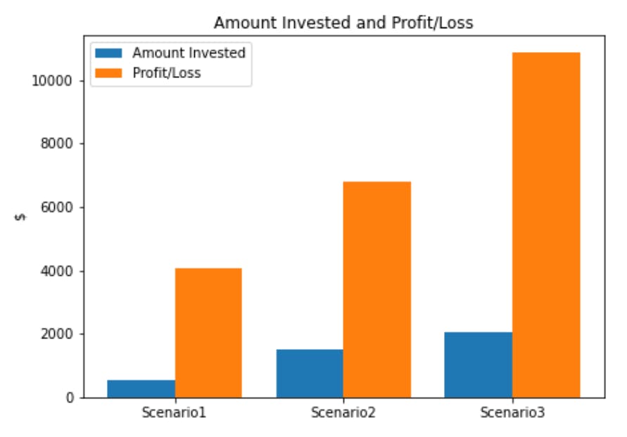
We can see that the amount invested in Scenario 3 is slightly higher than the amount invested in Scenario 2. However, the profit in Scenario 3 is significantly higher than in Scenarios 1 and 2.
ROI Comparison
plt.figure(figsize=(7,5))
plt.bar(strategy,roi,color='green')

plt.title("ROI Comparison")

plt.ylabel("ROI")
plt.plot()
plt.show()
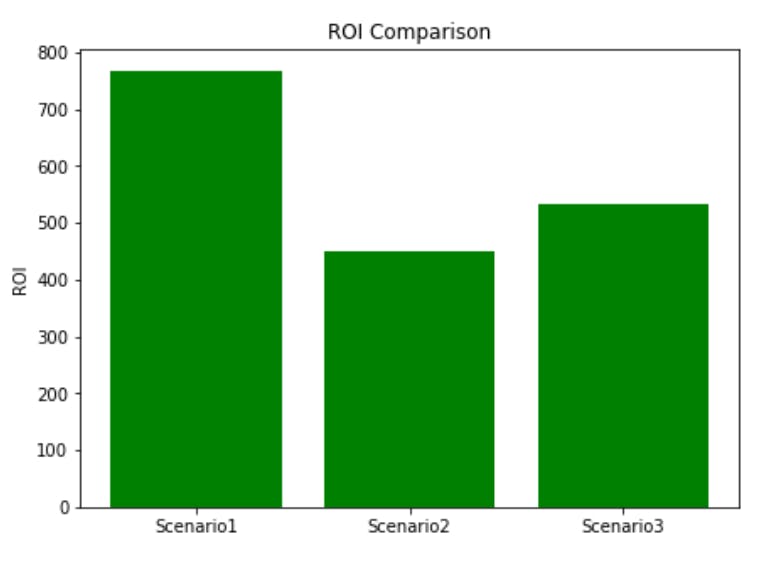
We can see that Scenario 1 has the highest Return on Investment. As a result, accumulating BTC during a bear market yields a higher ROI, followed by Scenario 2 and then 1.
BTC Accumulated
plt.figure(figsize=(7,5))
plt.bar(strategy,qty,color='gold')

plt.title("BTC Quantity Accumulated")

plt.ylabel("Quantity")
plt.plot()
plt.show()
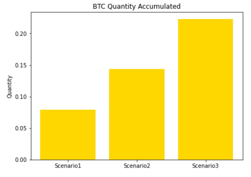
We can see that the quantity of BTC accumulated in Scenario 3 - during the bear and bull markets is the greatest. This is true because the accumulating period is longer in Scenario 3 as compared to Scenarios 1 and 2.
Average Buying Price
plt.figure(figsize=(7,5))
plt.bar(strategy,avg_buying_price,color='maroon')

plt.title("Average Buying Price")

plt.ylabel("Average Price ($)")
plt.plot()
plt.show()
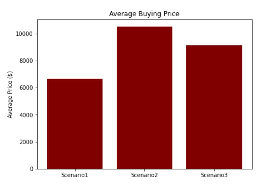
We can notice that the average buying price in Scenario 1 is the least, followed by Scenario 3 and Scenario 2. This is true since, Scenario 1 was during the Bear market and prices during the bear market are low. Scenario 2, we accumulated only during the bull market hence during bull market prices are high.
Conclusion
To summarize, an investor may make significant gains just by accumulating BTC at any period and holding it for the long term. However, if an investor wants to make the most of their money, they must adhere to a strategy. This is only one of the many investing strategies out there. However, this is NOT financial advise; all work done here is entirely for educational purposes. Before investing, an investor should perform their own research. Furthermore, this strategy can be used with other strategies to generate even better results.
Key Takeaways
- We have gathered data from CoinMetrics API.
- Next, we checked if the data is free from errors.
- Then we begin our analysis.
- We obtain the results for our three scenarios and then visualize them.
- From our analysis, Scenario 1 has the greatest ROI, followed by Scenario 3, and then Scenario 2.
- This is NOT FINANCIAL ADVICE.
Please feel free to connect with me and ask for any investing strategy or analysis you'd like me to perform. If you enjoyed my article and found it informative please follow. Thank you for your time.