Introduction

We all have a variety of stocks in our stock portfolio. Each individuals stock portfolio is different as it depends on an investors risk appetite, his likeness for that stock and that company, the stocks sector (industry the company operates in), the investors views of the macro environment, the investors goals and a number of other factors. Depending on these factors, an investor or an asset manager allocates particular stocks to their stock portfolio.

A stock portfolio is a basket of the stocks you have invested in. It basically refers to all the stocks an investor owns.

What is Portfolio Analysis

Portfolio Analysis is the process of analyzing your stock portfolio by comparing the returns of the stocks in the portfolio, checking portfolio diversification, asset correlation and much more. After analyzing your portfolio, investors or asset managers can make certain changes such as reallocating certain stocks, selling or buying other stocks in order to maximize your Return on Investment (ROI) and diversify the portfolio.

How to find stock ticker symbol

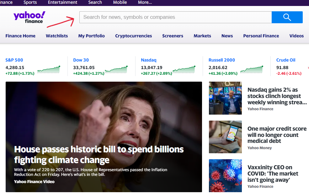
Since we will be using the Yahoo Finance API, it is essential to use the stock ticker symbols from yahoo finance site. You can visit the yahoo finance website by clicking here.

Once on the website, use the search box to search for the specific stock you own.

After selecting your stock, once on that specific stock page, the ticker should be displayed in circular brackets next to the stock name ().

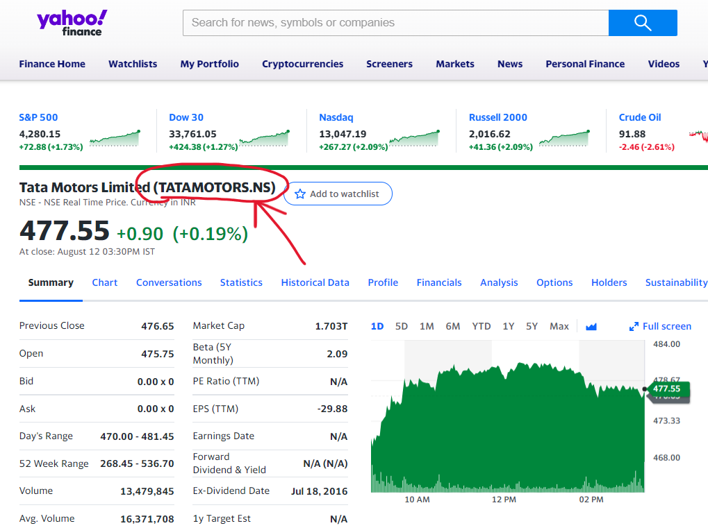
Note down each of your stocks ticker symbol into a list as done in "Manually Entering Stock Data" section.

Click here and here (API docs) to know more about the Yahoo Finance API.

Libraries Used

The libraries used in this project make it extremely simple to analyze your data. Installing these libraries is done using the pip command in the terminal:

pip install library_name

The libraries used are briefly described below:

• yfinance - Used for extracting stock data
• numpy - To make numerical calculations within grouped data simple
• pandas - To easily manipulate data in a dataframe
• matplotlib - To visualize your data
• seaborn - Used for data visualization
• datetime - To perform calculations on dates

Let's begin coding

Importing Libraries

import yfinance as yf
import numpy as np
import pandas as pd
import matplotlib.pyplot as plt
import seaborn as sns
import datetime as dt
from datetime import datetime

Manually Entering Stock Data

In this section, we will enter our stock data manually. Stock data includes our stock ticker symbol (from yahoo finance ONLY), shares we hold, price we bought the stock at, and the buying date of the share.

Visit the "How to find stock ticker symbol" section to find the stocks right ticker symbol.

stocks =['IRCTC.NS','TATAMOTORS.NS','LICI.NS','WIPRO.NS','INFY.NS','HDFCBANK.NS','RELIANCE.NS']
stock_holdings=np.array([10,15,7,20,5,3,4])
buying_price=np.array([748,248,825,414,1650,1535,2035])
dates=np.array(['2021-09-08','2021-08-16','2022-05-20','2021-03-01','2021-08-02','2021-02-01','2021-07-07'])

Stock Price and Sector

We will get our stock price and sector through the Yahoo Finance API.

price_stock_today=[] #to store stock price
sector=[] #to store stock sector

for i in stocks:
    asset=yf.Ticker(i) 
    price_stock_today.append(asset.info['regularMarketPrice'])
    sector.append(asset.info['sector'])

Basic Portfolio Calculations

amt_invested=np.multiply(stock_holdings,buying_price)

price_stock_today=np.array(price_stock_today)

stock_holdings_value=np.multiply(stock_holdings,price_stock_today)

stocks_profit_loss=stock_holdings_value-amt_invested

roi=(stocks_profit_loss/amt_invested)*100

Current_Portfolio_Value=sum(stock_holdings_value)
Total_invested=sum(amt_invested)
total_profit_loss=round(Current_Portfolio_Value-Total_invested,2)
total_roi=round((total_profit_loss/Total_invested)*100,2)

weight=np.divide(amt_invested,Total_invested)

The variables created are briefly described below:

• amt_invested - The total amount invested in each stock
• price_stock_today - The market price of one stock
• stock_holdings_value - The current value of each stock (Number of stocks x Market price of stock)
• stocks_profit_loss - The profit or loss of each stock
• roi - The return on investment of each stock
• Current_Portfolio_Value - The total value of our portfolio
• Total_invested - The total amount invested in our portfolio
• total_profit_loss - Portfolio's profit or loss
• total_roi - Portfolio's return on investment
• number_days - The number of days we held our stock for (Created in the code below)

Calculating Number of Days

We will calculate the total number of days we are holding each stock in our portfolio.

buy_date=[]

#converting each date from 'string' to 'datetime' datatype and storing in a list
for i in dates:
    buy_date.append(datetime.strptime(i, "%Y-%m-%d"))

#converting list to numpy array for easy calculations
buy_date=np.array(buy_date)

#finding difference between buying date and todays date

number_days=[]
for i  in buy_date:    
    number_days.append((dt.datetime.now()-i).days) # .days is an in-built function which returns only number of days

Displaying Stock Details and Portfolio Results

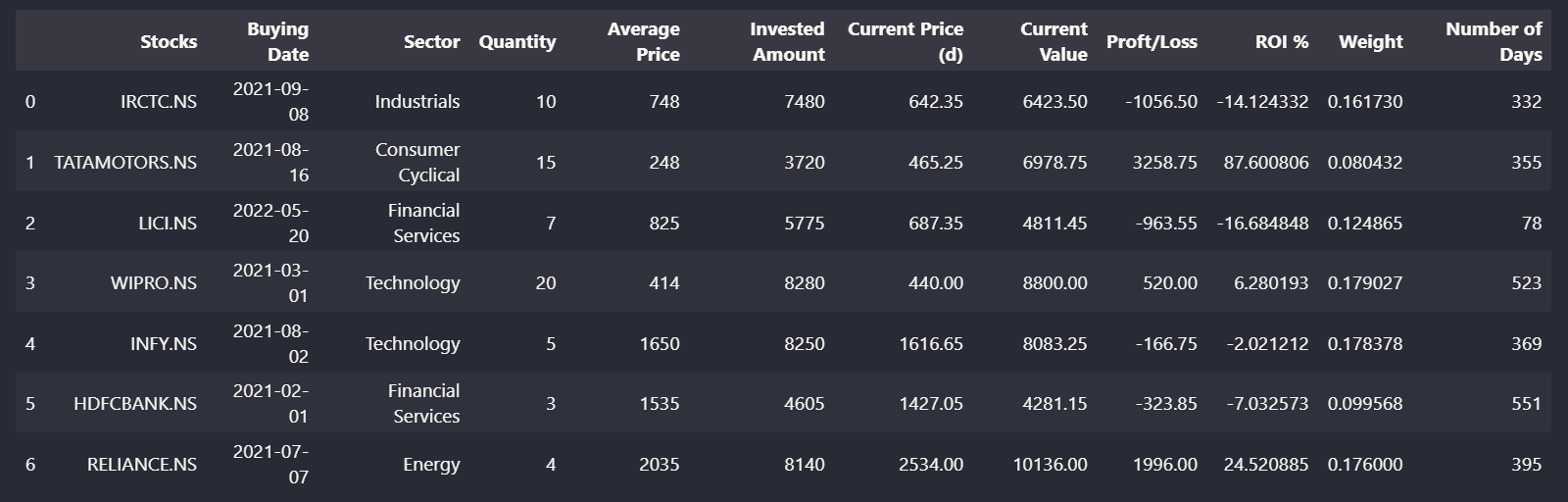
We will first store the details of the stocks we own in a dataframe. We will then print our dataframe to view our stock details. Following that, we will print our entire portfolio's results.

Creating the Dataframe

df=pd.DataFrame() #Creating empty dataframe

df['Stocks']=stocks
df['Buying Date']=dates
df['Sector']=sector
df['Quantity']=stock_holdings
df['Average Price']=buying_price
df['Invested Amount']=amt_invested
df['Current Price (d)']=price_stock_today
df['Current Value']=stock_holdings_value
df['Proft/Loss']=stocks_profit_loss
df['ROI %']=roi
df['Weight']=weight
df['Number of Days']=number_days

Displaying Stock Details

print(df)

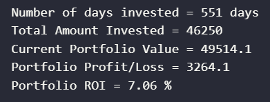
Displaying Portfolio Results

print("Number of days invested =",max(df['Number of Days']),"days")
print("Total Amount Invested =",Total_invested)
print("Current Portfolio Value =",Current_Portfolio_Value)
print("Portfolio Profit/Loss =",total_profit_loss)
print("Portfolio ROI =",total_roi,'%')

Portfolio Visualization

ROI Analysis

color=['Grey','Blue','Red']
plt.figure(figsize=(20,7))
plt.bar(df['Stocks'],df['ROI %'],color=color)

plt.title("Stocks ROI")
plt.ylabel("ROI")

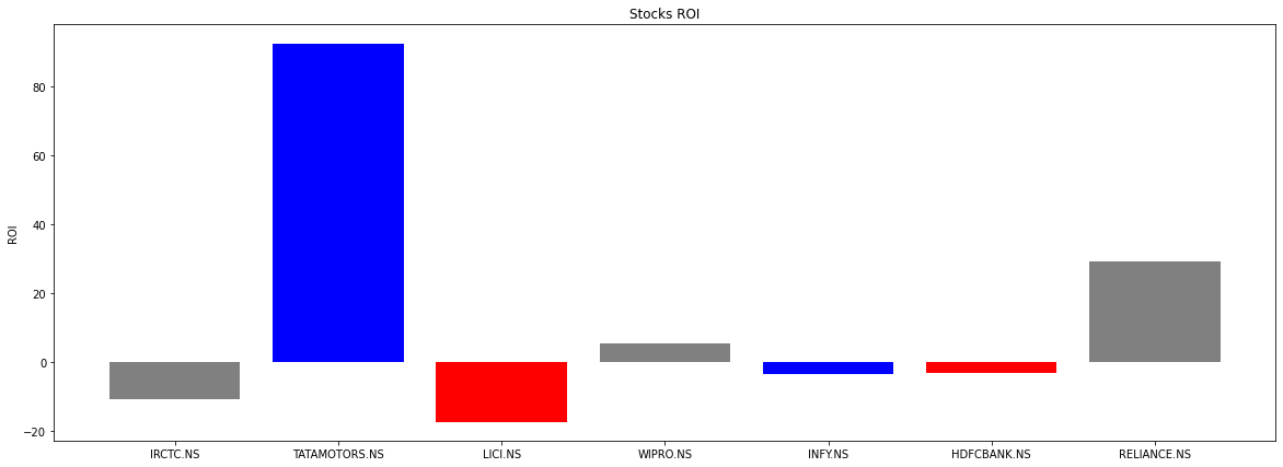
We can notice, Tata Motors has given us the highest ROI whereas LIC has given us the lowest.

Amount Invested and Profit/Loss

plt.figure(figsize=(20,7))

x_axis = np.arange(len(stocks))

plt.bar(x_axis -0.2, amt_invested, width=0.4, label = 'Amount Invested')
plt.bar(x_axis +0.2, stocks_profit_loss, width=0.4, label = 'Profit/Loss')

plt.xticks(x_axis, stocks)

plt.legend()

# Displaying

plt.title("Amount Invested and Profit/Loss")
plt.ylabel("Price (Rs)")
plt.show()

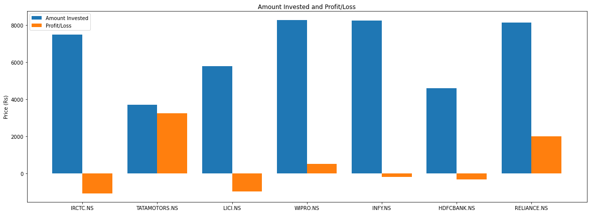
We can see from our above results that we have invested the most amount in Wipro, Infosys, Reliance, and IRCTC. Only Wipro is currently profitable from these investments; the others are currently in loss. Furthermore, we can see that despite investing the least amount in Tata Motors, we have the highest profit.

ROI and Number of Days

plt.figure(figsize=(20,7))

x_axis = np.arange(len(stocks))

plt.bar(x_axis -0.2, roi, width=0.4, label = 'ROI',color='pink')
plt.bar(x_axis +0.2, number_days, width=0.4, label = 'Number of Days',color='grey')

plt.xticks(x_axis, stocks)

plt.legend()

# Display

plt.title("ROI and Number of Days")
plt.ylabel("Number of Days")
plt.show()

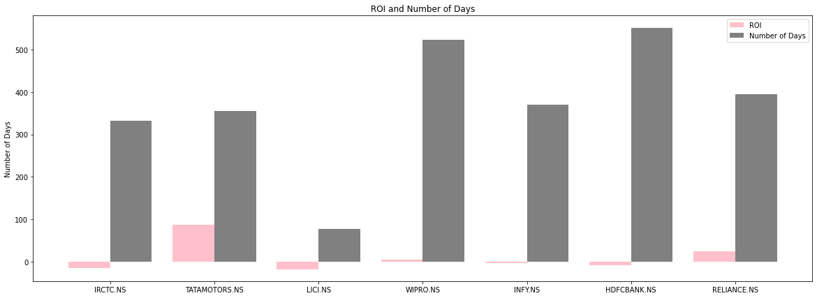We can see from our above output that HDFC and Wipro are stocks that we have held for a long period. Despite this, our profit for Wipro is quite little, whereas we are in a loss for HDFC. Perhaps, its time to change some of our stock holdings and allocations?

Number of Shares for each Stock

plt.pie(df['Quantity'],labels=df['Stocks'],shadow=True,autopct='%1.1f%%')
plt.title('Quantity')
plt.show()

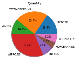We can see that we own the most shares of Wipro and the least number of shares for HDFC bank.

Portfolio Diversification

Diversification refers to investing in a number of different assets. Here in our case investing in a number of different cryptocurrencies.

plt.pie(df['Weight'],labels=df['Stocks'],shadow=True,autopct='%1.1f%%')
plt.title('Diversification')

plt.plot()
plt.show()

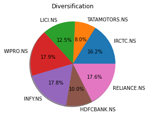We can see from the above figures that our largest holdings are Wipro, Infosys, and HDFC Bank. Tata Motors is our smallest holding.

Sector Wise Diversification

Each stock has its own sector such as Finance, Energy, Technology and many more. We have got the sector of each stock from the Yahoo Finance API.

We can see from our stock details dataframe df that several stocks operate in the same sector, hence we need to calculate the count of each sectors. We will create a seprate dataframe for our sectors.

Sector Dataframe

sec=df.groupby(['Sector']).size() 
sec=pd.DataFrame(sec)
sec.head()

The groupby function, groups the sectors and returns the count of each sector.

We can see that multi-indexing has occurred. To resolve this, we must reset our index. We can accomplish this using the code below.

sec.reset_index('Sector',inplace=True) #resolve multi-indexing
sec.columns=['Sector','Count'] #changing column names
print(sec) #displaying our sector dataframe

Sector Diversification

plt.pie(sec['Count'],labels=sec['Sector'],shadow=True,autopct='%1.1f%%')
plt.title('Sectors')
plt.show()

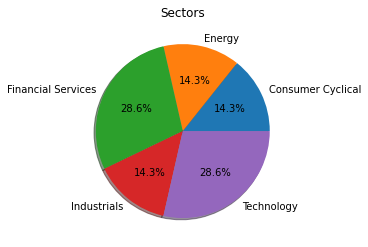Here, we notice that the majority of the stocks we own, operate in the "Financial Services" and "Technology" sector.

Further Analysis

Obtaining Stock Historical Data

d=[]

for i in range(len(stocks)):
    a = yf.Ticker(stocks[i])
    hist = a.history(start=dates[i])['Close'] #return type series
    data = hist.to_frame() #convert series to dataframe

    #data.set_index('Date',inplace=True)
    data.rename(columns={'Close':stocks[i]},inplace=True)
    d.append(data)

hist=pd.concat(d,axis=1)
hist.head()

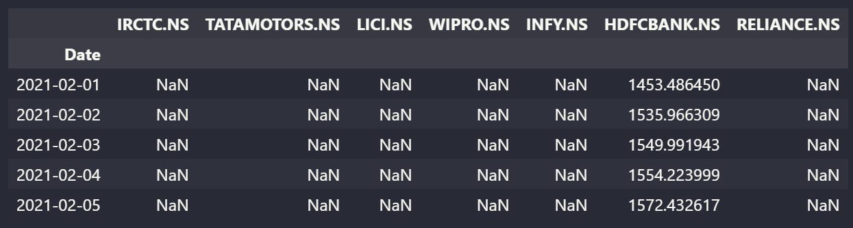
In the above code, we have extracted the historical closing price of our stocks from the time we have purchased the particular asset, by using the Yahoo Finance API.

After the above code has been executed, we notice that multi-indexing has occured. Hence we need to resolve this. We can do so by executing the code below.

hist=hist.reset_index(level=['Date'])#multi indexing

Now if we execute the .head method, we will notice multi-indexing has been eliminated.

Comparing Stock Price

plt.figure(figsize=(20,7))

for i in range(len(stocks)):    
    plt.plot(hist['Date'],hist[stocks[i]],label=stocks[i])

plt.legend()
plt.title("Stock Holdings Performance")
plt.ylabel("Price (Rs)")
plt.xlabel("Date")
plt.plot()
plt.show()

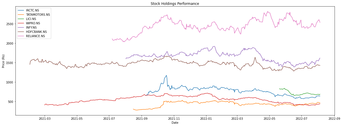
There's a gap between the stocks, since we have bought the stocks at different dates.

Stock Correlation

In this section, we will compare the correlation of the stocks in our portfolio.

• Positive Correlation - A positive correlation indicates that if the price of one stock rises, the price of the other stock will most likely rise as well and vice versa (price falls, price rises). The two variables (stocks) are related to each other.

• Negative Correlation - A negative correlation indicates that if the price of one stock rises, the price of the other stock will most likely fall and vice versa (price falls, price rises). The two variables (stocks) are not related to each other.

• The more the correlation value is towards 1, the more likely the stock will follow the same direction.

• The more the correlation value is towards -1, the more likely the stock will not follow the same direction.
• A correlation value of 0 indicates there is no correlation between two variables (stocks).

We first will drop all the Null values of our stock price data (hist dataframe) to get accurate results and store this in another dataframe.

no_null=hist.dropna()

We now will find the correlation.

c=no_null.corr()
plt.figure(figsize=(10,7))
sns.heatmap(data = c,annot=True)

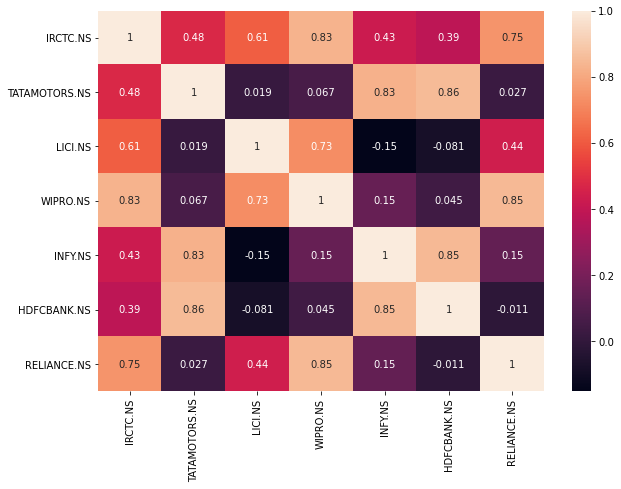
Here we can notice, the lowest correlation (-0.059) is between HDFC and Reliance. This is true since HDFC is in the Financial Services sector whereas reliance is in the Energy sector.

Many of the times stocks trading in different sectors too are correlated such as in our case you can notice IRCTC (Industrials) and Wipro (Technology) has the highest correlation of 0.84.

We can also notice, Wipro and Infosys which operate in the same sector i.e Technology are highly correlated (0.81).

Normally, a strong portfolio diversification requires a low number of highly correlated stocks. The majority of the stocks in our portfolio are not highly correlated which indicates our portfolio is well diversified.

Stock Volatility

In this section, we will compare the volatility of the stocks in our portfolio's daily returns. Volatility is defined as the major change in price (in percentage) of any asset over time.

date=hist['Date'] #Storing Dates
percent_change=(hist.drop('Date',axis=1)).pct_change()

If we print percent_change, we may notice we have a number of Null values. This is true since, we bought our stocks at different intervals of time.

plt.figure(figsize=(15,8))

for i in percent_change.columns.values :
    plt.plot(date,percent_change[i] ,label = i)

plt.legend(loc = 'upper right')
plt.title('Volatility')
plt.xlabel('Date')
plt.ylabel('Daily Simple Returns')

plt.show()

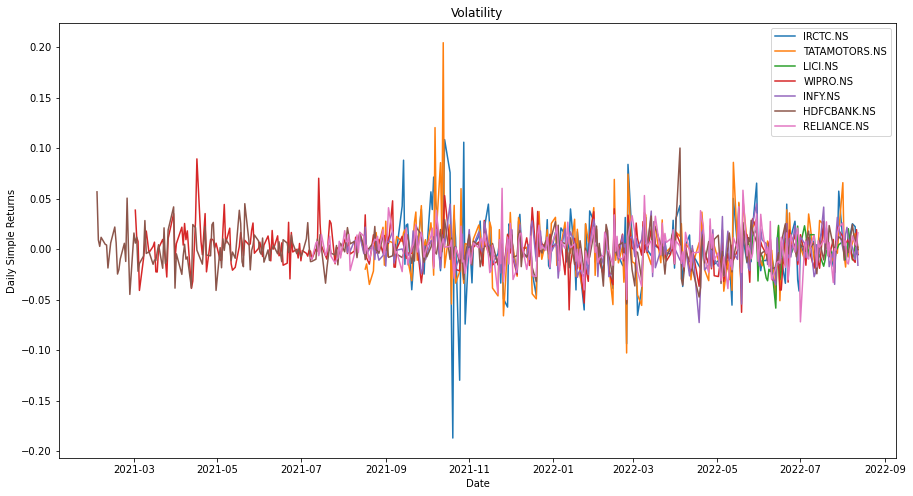
From the above chart, we can see that the blue line (IRCTC) has dropped the most (18% in a day), while the yellow line (Tata Motors) has increased the most (20% in a day).

Furthermore, we may notice the yellow line (Tata Motors) has been having some of the largest swings in both direction. Thus, signifying Tata Motors is a volatile stock.

Portfolio Performance

Portfolio Value Overtime

In this section, we will calculate our entire portfolio value over time from the time we bought our first stock.

hist.fillna(value = 0,inplace = True) #Replaicing Null Values with 0

s=0
for i in hist:    
    s=0
    for j in range(len(stocks)):
        p=stock_holdings[j]*hist[stocks[j]] #calculating each stock value
        s=s+p #sum of each stock
    hist['Portfolio Value']=s

Visualizing Portfolio Value

plt.figure(figsize=(20,7))
plt.plot(hist['Date'],hist['Portfolio Value'])

plt.title("Portfolio Value Overtime")
plt.ylabel("Price (Rs)")
plt.xlabel("Date")

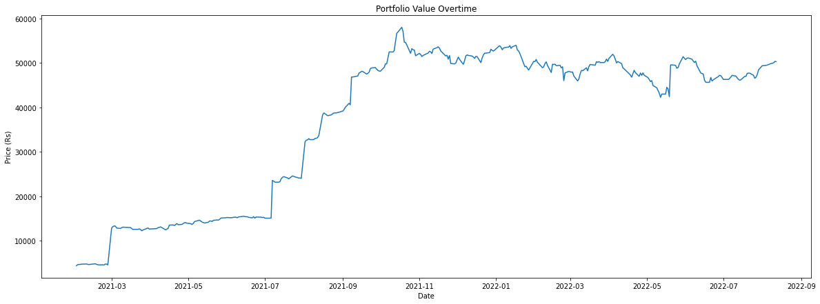The sudden spikes in our portfolio is due to addition on new stocks to our portfolio.

Portfolio Statistics

plt.figure(figsize=(10,7))
hist.boxplot('Portfolio Value')

plt.title("Portfolio Statistics")
plt.ylabel("Price (Rs)")

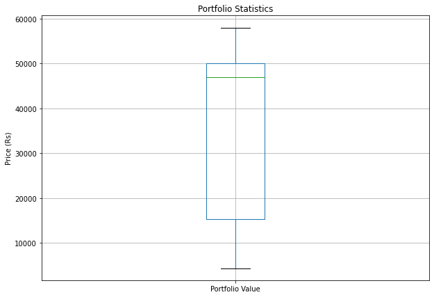Here we see, the maximum value our portfolio reached is ~58,000, the minimum value of our portfolio was ~4,000 (we began investing at this time)and our median value is ~47,000.

Portfolio Comparison with Indices

In this section, we will compare our Portfolio cumulative return with indices such as NIFTY 50, Gold, SENSEX and S&P 500.

Indices are basically a measure of the performance of a group of stocks.

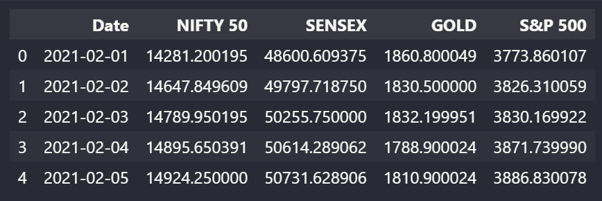
Gathering Index Data

index_data=[]

indexes=['NIFTY 50','SENSEX','GOLD','S&P 500']
index_ticker=['^NSEI','^BSESN','GC=F','^GSPC'] #yahoo finance tickers

for i in range(len(index_ticker)):
    nse=yf.Ticker(index_ticker[i])
    data=nse.history(start='2021-02-01')['Close'] 

    data=data.to_frame()
    data.rename(columns={'Close':indexes[i]},inplace=True)
    index_data.append(data)

df_index=pd.concat(index_data,axis=1)

df_index=df_index.reset_index(level=['Date']) #since multi indexing occured
df_index.dropna(inplace=True)
df_index.head()

In the line data=nse.history(start='2021-02-01')['Close'] , the start date refers to the date we bought our first stock.

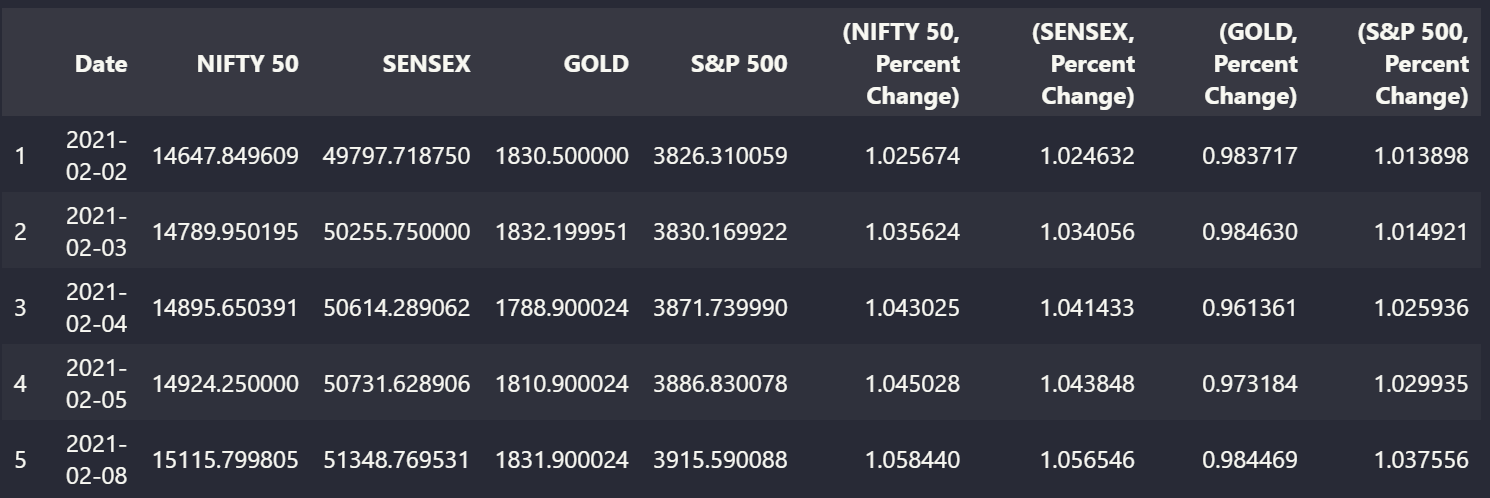
Calculating Cumulative Returns

First, we will calculate the cumulative returns for our indices.

l=df_index.columns

for i in range(1,5): #beginning from 1 since we do not want to perform calculations on date
    df_index[l[i],'Percent Change']=(df_index[l[i]].pct_change()+1).cumprod()

df_index.dropna(inplace=True) #Since first row value becomes NULL
df_index.head()

Now we will calculate the cumulative returns of our Portfolio Value.

cummulative_returns=((hist['Portfolio Value'].pct_change())+1).cumprod()

Comparing Cumulative Returns - Portfolio Vs Indices

Since our portfolio's cumulative returns are much higher than the cummulative return of each index, we are required to use a subplot and a twin axis.

l=df_index.columns
plt.rcParams['figure.figsize']=(20,7)
fig, ax1=plt.subplots()
ax2=ax1.twinx()

y=df_index['Date']

for i in range(5,9):
    ax1.plot(y,df_index[l[i]],label=l[i-4])

ax2.plot(hist['Date'],cummulative_returns,color='Black',label='Portfolio C. Return')

h1, l1 = ax1.get_legend_handles_labels()
h2, l2 = ax2.get_legend_handles_labels()
ax1.legend(handles=h1+h2, labels=l1+l2, loc='upper left')

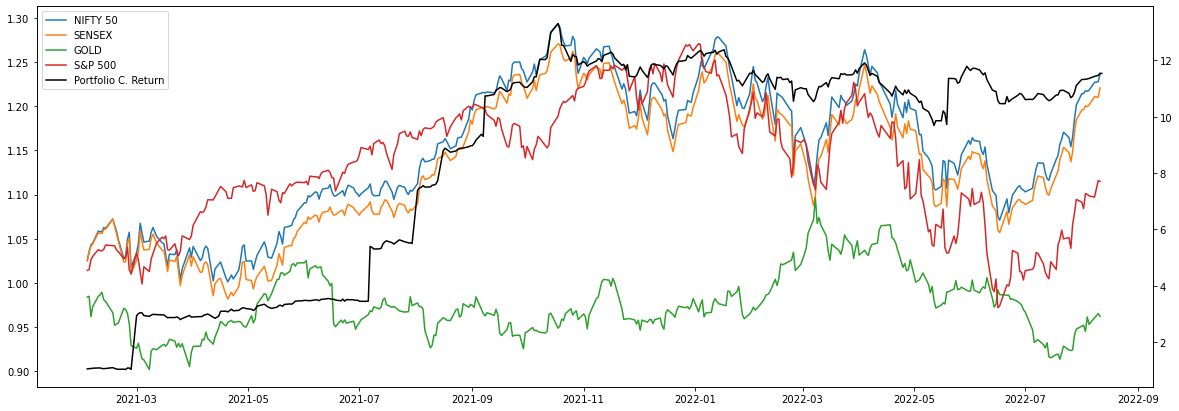
The y-axis on the right side is our Portfolio's cumulative return whereas the y-axis on the left side is the cumulative return of the indexes.

We can notice our portfolio has outperformed a number of indices by a huge number.

Portfolio Monthly Performance

To calculate our monthly performance, we need to create three additional tables in our dataframe - 'Year', 'Month' and 'YearMonth'.

Creating Additional Tables

hist['Month']=hist['Date'].dt.month
hist['Year']=hist['Date'].dt.year

If we run the .head() method, we can notice two additional columns. Now we simple cannot plot the monthly returns since we have data from 2021 and 2022, and this data will consist of two months meaning Feb 2021 and Feb 2022. Hence we need to create an additional column which distinguishes these months.

def getYearMonth(s):
    s=s.strftime("%m/%d/%Y")
    return s.split("/")[0] + "-" + s.split("/")[2]

hist['YearMonth'] = hist['Date'].apply(lambda x: getYearMonth(x))

The getYearMonth() function we have created, will return to us a result such as '02-2021' and '02-2022' for each month and year.

Data Manipulation

Now we have created our three additional columns. Our next step is to group our data by 'YearMonth' since we are calculating our portfolio's monthly performance. We are storing this grouped data in another variable 'a'.

a=hist.groupby(["YearMonth"]).mean()
a.reset_index('YearMonth',inplace=True) #resolving multi-indexing

Next we will sort 'a' according to Year and Month and store this sorted dataframe in another variable 'b'.

b=(a.sort_values(by=['Year','Month']))

Visualizing Portfolio's Monthly Return

plt.bar(b['YearMonth'],b['Portfolio Value'],color='darkgreen')

plt.title("Portfolio Monthly Value")
plt.ylabel("Price Rs")
plt.xlabel("Months")

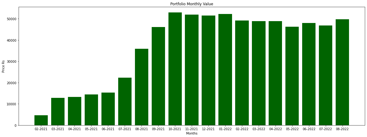
We can notice in October, our Portfolio's value was the highest. From October, our Portfolio is in a consolidation phase.

Conclusion

Yes I know, this a looong blog. But if you have stuck till the end I can assure you that you would have grasped a good amount of knowledge and ideas. This project is NOT FINANCIAL ADVICE. All the work done in this project is purely for educational purposes. Please feel free to add your own stock holdings as done in the "Manually Entering Stock Data" section and analyze your portfolio. Stay tuned for an upcoming project on "Cryptocurrency Portfolio Analysis".

If you have found this project informative in any way please comment below and considering following.Thank you for your time.